Priority Interdependencies
Based on models of task progress, population and consumption, and priorities, the following relationships are assumed:
| Relationship | Definitions |
hself = F / ( uh * F + Fmin ) = Env / Envtot |
|
| Fe = P * F |
|
| h = i4 * Fe4 - i3 * Fe3 + i2 * Fe2 + i1 * Fe |
|
Lself = F / ( uL * F + frate )
|
|
| Ltot = [ FeTotal - ( Fe + FeMin ) ] / ( dFe/dt ) |
|
| S = -b1 * Fe + b0 |
|
| Lspecies = ( FeTotal - Fe ) / ( dFe/dt ) |
|
| Q = 1 - (1 - E )t/tmin |
|
| SUM(Prioritygoal)1 to g = (1 - Priority0)g |
|
| Qgoal = 1 - ( 1 - Egoal )T |
|
| Effect = [ (P - N) * XP + N * XN ] / P |
|
Key aspects can be summarized by the following rules of thumb:
| INCREASE | TO DO THIS |
|
|
|
|
|
|
|
|
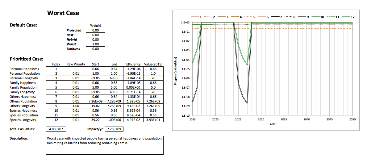
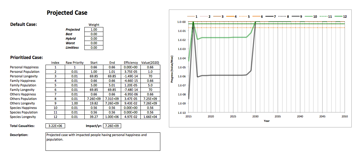
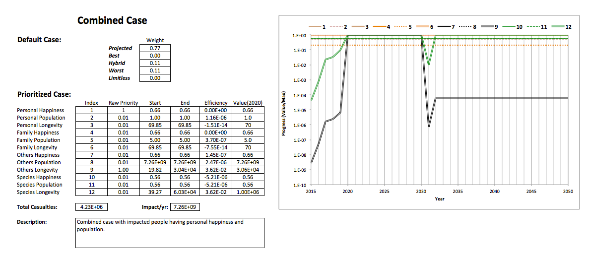
The following images show the results of simulations using several Half-World scenarios.
The total ecological resources are fixed at their current estimated value, and high priority is placed on others longevity, which is influenced by getting a number of people to adopt the same personal goals ("impact"). Graphs show the trajectories of progress for all goals (identified by index numbers) on a logarithmic scale, with each year marked at the middle of the year.
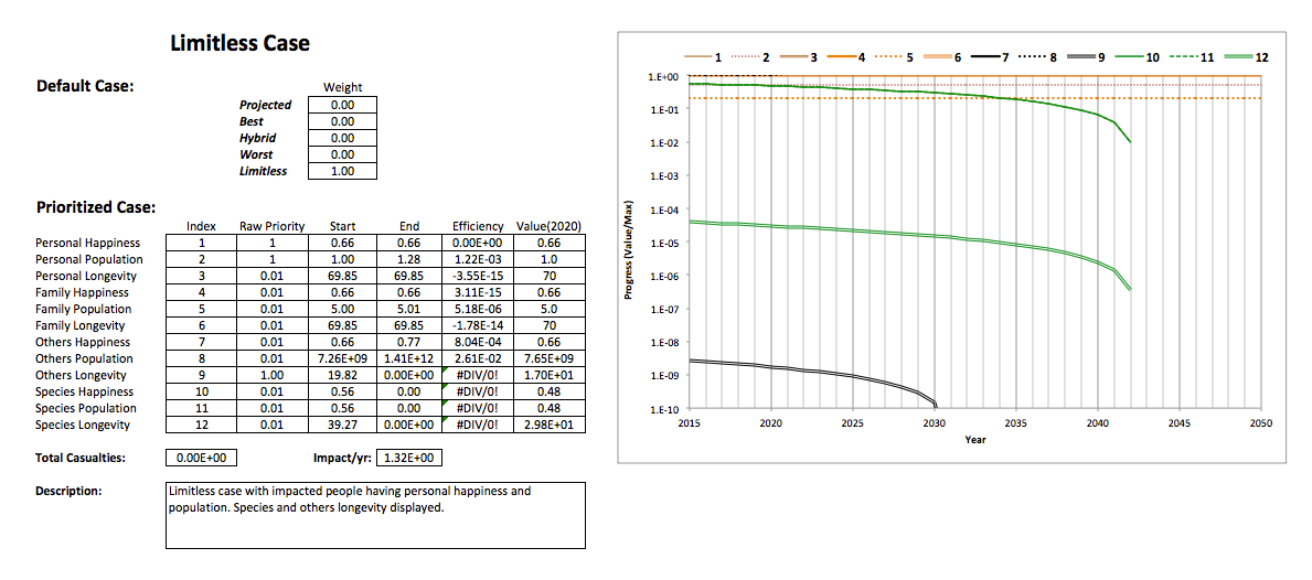
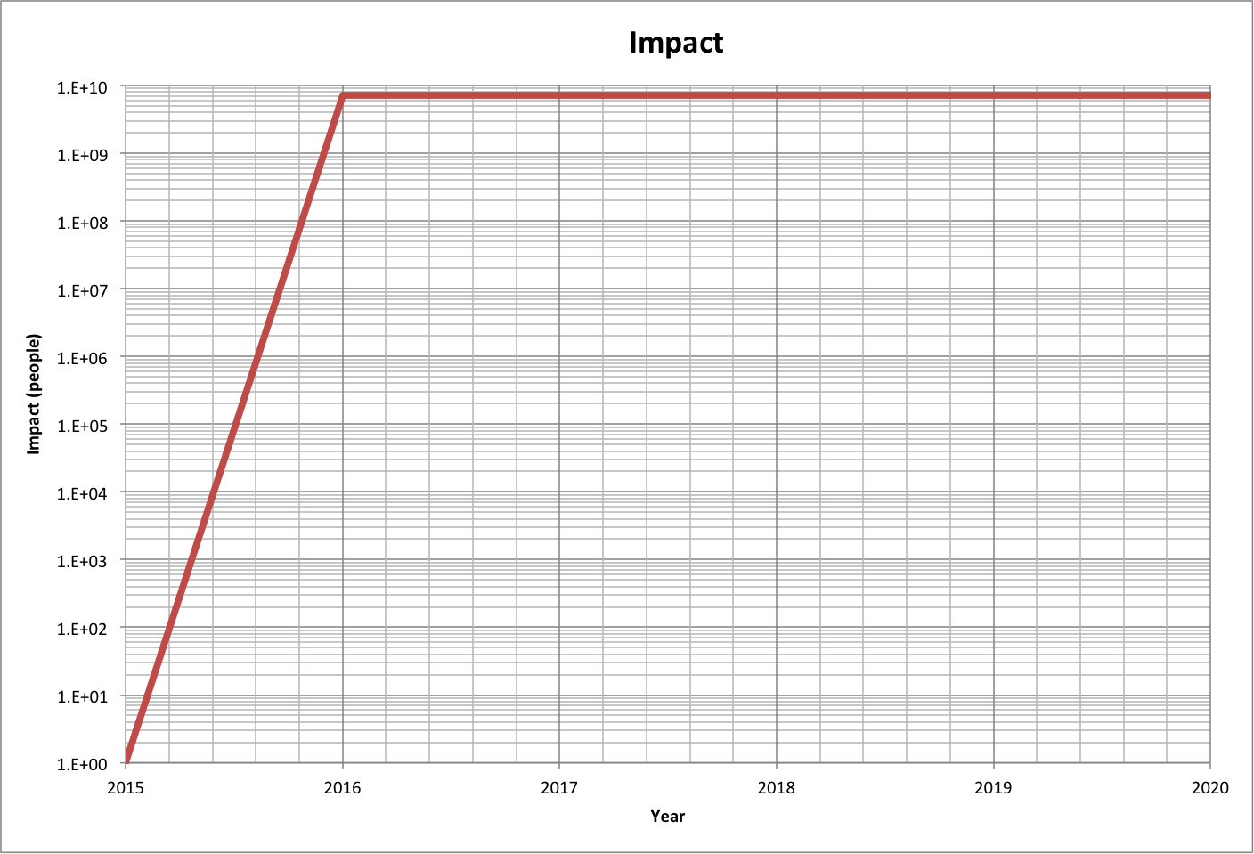
The following graph shows impact as a function of time for full effect (7.26E+09/yr):
While the graphs above assume that there is built-in impetus to follow the trajectories in the Half-World scenarios (which are modified by the changes due to priorities), the following graphs display how population and footprint are constrained if enough ecological resources are left to support the species we depend on for basic survival. That is, Fe + FeMin < FeTotal - FeMin, and therefore
- Varying F, then P < [ Pcritical = FeTotal / ( F + 2 * Fmin ) ]
- Varying P, then F < [ Fcritical = FeTotal / P - 2 * Fmin ]
The next graph begins with values of population (Pstart) and footprint (Fstart) in mid-2015, and plots
- P vs. F = P / Pstart on X-axis, Fcritical / Fstart on Y-axis
- F vs. P = F / Fstart on X-axis, Pcritical / Pstart on Y-axis
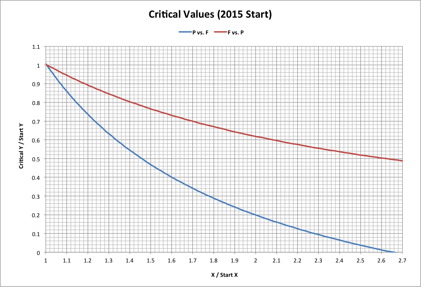
The following graph plots critical values of P and F as above, but over a broader range. Here, Pstart = 1 and Fstart = Fmin.
Note that, in 2015, P / Pstart = 7.26E+09 and F / Fstart = 3.29. Roll over the image for a close-up.
.png)
Corresponding happiness values are shown below, where
- P vs. Critical h = P / Pstart on X-axis, happiness at Fcritical on Y-axis
- F vs. h = F / Fstart on X-axis, happiness at F on Y-axis
Current (2015) happiness is 0.66.
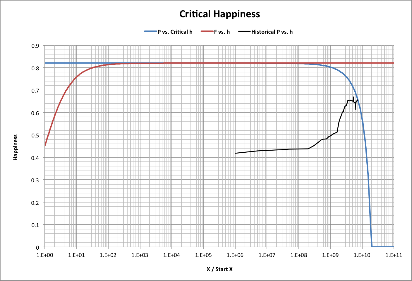
Historical values of footprint and population from 1950-2015 are superimposed on the critical values (with Pstart = 1, Fstart = Fmin) in the graph below. Roll-over the image to see P vs. F.
Also shown are results of a simulation that starts with F and P for 1950 and takes the following steps 2500 times:
- Calculate current F limit.
- Move F toward the limit as a fraction of the distance to it, with the fraction equal to a random number (between 0 and 1) times an efficiency of 0.002.
- Calculate the new P limit.
- Move P toward the limit as a fraction of the distance to it, with the fraction equal to a random number (between 0 and 1) times an efficiency of 0.01.
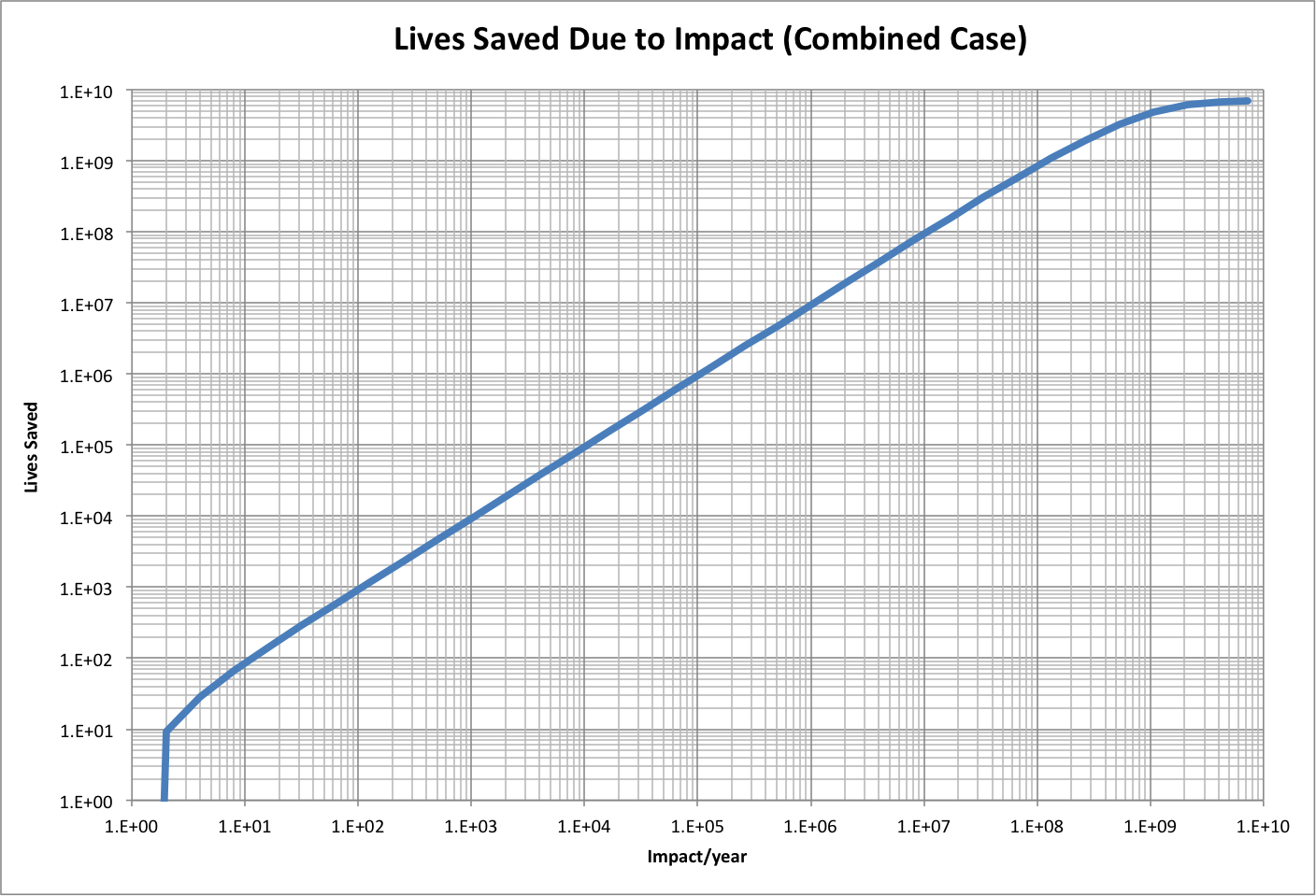
The following graph takes critical population values and calculates the corresponding critical footprints, then calculates happiness from the results to derive a plot like that used in the simulations of population and consumption used in version 4 of the Population-Consumption model.
For a discussion, see the following:
- Impacts (Idea Explorer blog)
- Action Time (Land of Conscience blog)