Normal Expectations

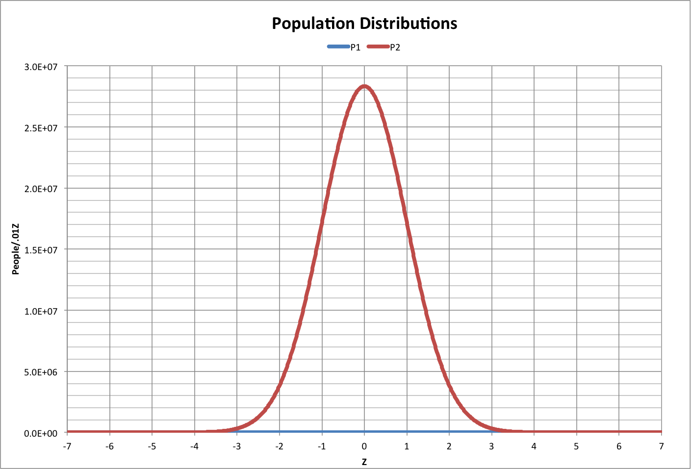
Most characteristics of a population such as ours are expected to be randomly distributed as a histogram approximating the "normal distribution" or "bell curve." This distribution is shown below for the population at the beginning of civilization at year -10000 (P1) and the year 2013 (P2):

The width of the distribution depends on the size of the population, since there is only one person at each end (tail). Here, the width is defined by the values of Z where the sum of the area under a tail equals 1. For example, in the year -10000, when the population was 1 million people, the distribution fell in the range -4.75 < Z < 4.75, where there was one person to the left of Z = -4.75 and one person to the right of Z = 4.75.

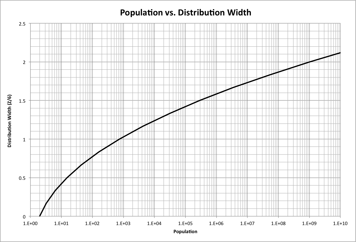
Under most practical circumstances, distributions have a maximum range of -3 < Z < 3, or a width of 6. Using a width of 6 as a standard width, the width as a function of population P can be approximated by the following, which is graphed below (roll over image to see corresponding Z values):

Width(Z/6) = 1.79898811035184*log(P)² + 7.35033302031070E-01*log(P) + 3.35628512083268E-01

Using this relationship, we can calculate how the width has changed over time and compare it to what it was at the beginning of civilization:

We can use this to estimate the distributions for characteristics that are dependent on the population distribution.

In general, the width for a characteristic X will be twice the difference between the average and the minimum value. The standard deviation (SD) allows us to translate any such distribution into values of Z:

Width(X) = Xmax - Xmin = 2 * (Xave - Xmin)

SD = Width(X)/Width(Z)

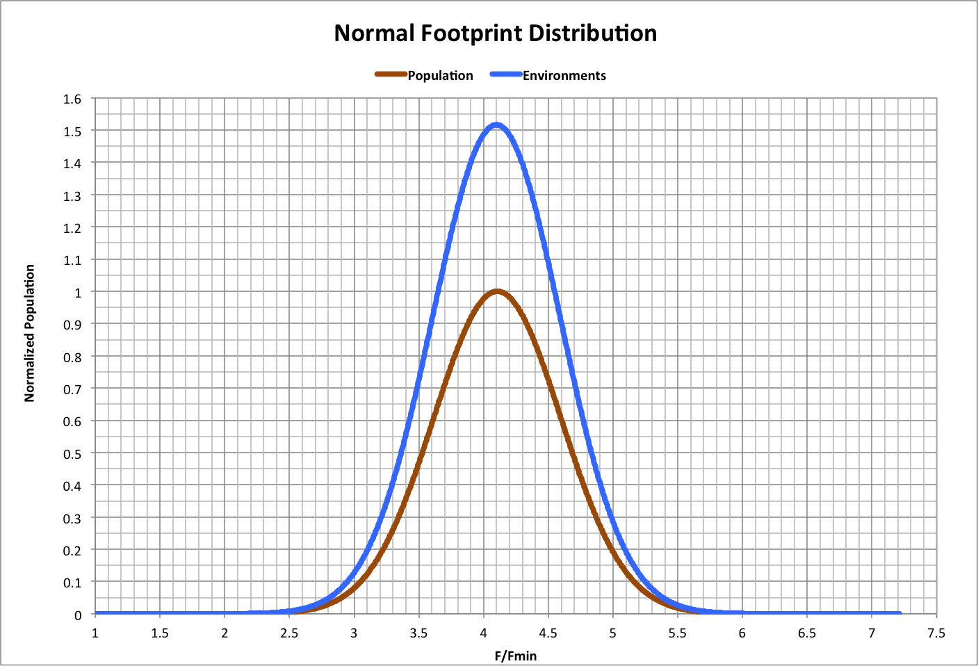
For example, the following is a graph of the expected average and standard deviation for the ecological footprint (as a multiple of the minimum footprint, Fmin) over time, where the distribution is expected to have the same width (units of Z) as the population, but with the average having moved so that the minimum value stays constant. Roll over the image for a close-up.

Note that the standard deviation SD (which is the equivalent F/Fmin for one unit of Z) has leveled off at about 0.5, corresponding to a global footprint of more than 1 Earth/year for the middle ~2/3 of the population (-1 < Z < 1) beginning in 2005, as shown below.

The following graph shows the expected distribution of the footprint in 2013, along with the environments (defined in PCM v4) associated with the happiness derived from the footprint:

If this distribution were accurate, then the maximum footprint should have been only be about 76% greater than the average in 2013, as shown below:

We know, of course, that the maximum is actually several times the average, the footprint distribution is not truly random, and the reason why (from PCM v4): the environments distribution is interfering with the population distribution and therefore distorting the happiness (and consequently the footprint) across the population.

If, however, the footprint distribution was as shown above, economic activity (Gross World Product per person) and wealth per person would also have normal distributions, based on the observations that:

GWP is propotional to (h * P)²
Weath is proportional to (h * P)³

The result for 2013 is graphed below:

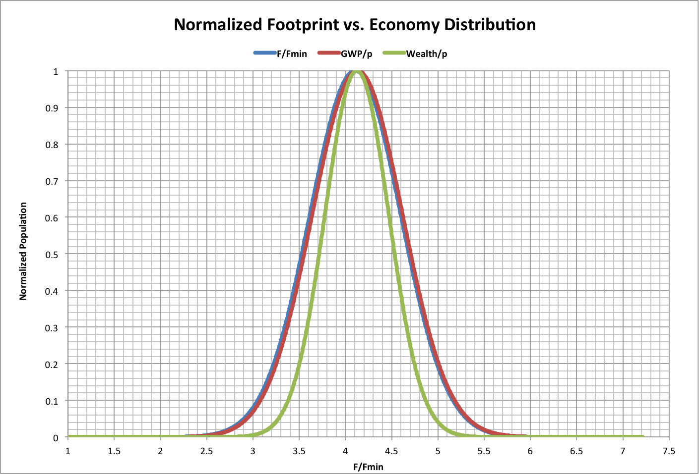
Note that this wealth distribution is what would be expected if it was normally distributed, which it is not, and tends to favor the population closer to the average.

For a discussion of this topic, see the blog "Changing People."